Deep Learning : Hello World
The internet regards the MNIST dataset as a sort-of “hello world” in the deep learning world so it seem’s a good starting point for getting to know the basics of various deep learning techniques and tools.
Problem Description
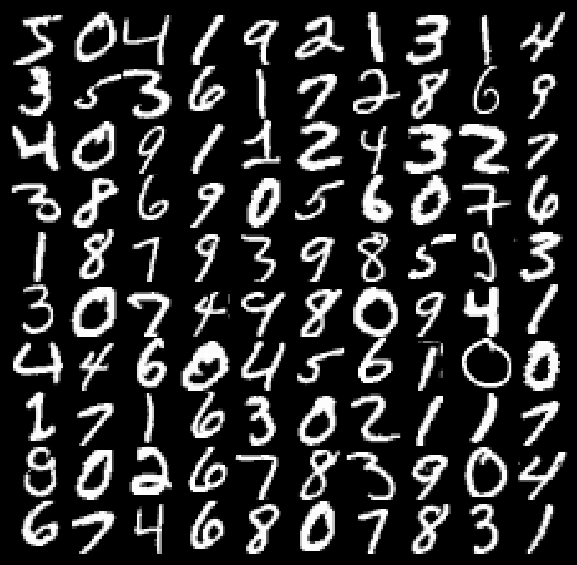
The MNIST dataset is a well-known collection of images of handwritten digits created by Yann Lecun for the purpose of developing and evaluating handwriting recognition systems. The dataset consists of about 60000 training images and 10000 test imatges which have been aquired from a variety of scanned documents and have been normalized in size and centered.
Each image represents a handwritten digit (0-9) and conists of 28 x 28 (784) pixels, each containing a value between 0 and 255 representing the grayscale pixel intensity. In addition the images are in white on black format ( meaning that the background has the highest pixel intensity).
For this project we will train a simple and a more complicated model to see if we can achieve something close to 99% accuracy ( according to the website, the most advanced convolutional neural network techniques are able to achieve a loss of just 0.23%)
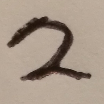
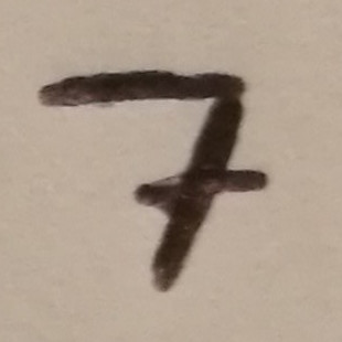
We will also test the models on our own data so i’ve written the year 2017 on a piece of paper, so at the end we can feed that into our system to see if it is able to interpret the digits.
Now we have the facts, let’s get started…
Setting up the Tools
The first step is to choose which tools and libraries to use.
I’ve gone with the popular choice of Keras with a Tensorflow backend. Keras is an intuitive python API for neural networks that enables faster prototyping of neural networks by promoting clean and minimal code. It can be configured with a number of popular deep learning libraries, but we have chosen Tensorflow for it’s popularity and compatibility.
For the purposes of this project the hardware requirements are not so important as models we will develop are not going to be very complicated, however if you intend on progressing to more complicated models and/or problems it might be worthwhile investing in a cloud GPU instance or a self built deep learning rig if you don’t want to be sitting around for hours waiting for your model to train.
Assuming you are using linux, the simplest way to get started is to use a pre-configured docker image containing all the tools we will need.
First install docker, or nvidia-docker if you wish to make use of an nvidia gpu.
Once you have installed docker, then simply find an appropriate docker image such as https://hub.docker.com/r/ermaker/keras-jupyter/ and run it.
$ docker pull ermaker/keras-jupyter
$ docker run -d -p 8888:8888 -e KERAS_BACKEND=tensorflow ermaker/keras-jupyter
Now we launch a bash session in the docker container and launch a new jupyter notebook. A jupyter notebook is a popular way of interacting with python code using the web browser and conveniently could allow you to develop code remotely from the backend.
$ docker exec -it <containerIdOrName> bash
$ mkdir mnist_project
$ cd mnist_project
$ jupyter notebook
Now we just copy the url provided into a web browser to begin developing (note the port forwarding for port 8888 has already been done for us in the docker run command).
Getting Started
An added benefit of using keras is that it already includes MNIST data, so loading it into your project is as simple as the following (provided that your machine has access to the internet)
from keras.datasets import mnist
#keras will automatically downlhoad the dataset
(x_train, y_train), (x_test, y_test) = mnist.load_data()
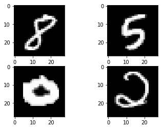
We can use matplotlib to view some randomly picked examples
import matplotlib.pyplot as plt
import random

#get the size of the dataset
train_size = len(x_train)

#set the seed so our random tests are reproducible
random.seed(49)

plt.subplot(221)
plt.imshow(x_train[random.randint(0, train_size-1)], cmap=plt.get_cmap('gray'))
plt.subplot(222)
plt.imshow(x_train[random.randint(0, train_size-1)], cmap=plt.get_cmap('gray'))
plt.subplot(223)
plt.imshow(x_train[random.randint(0, train_size-1)], cmap=plt.get_cmap('gray'))
plt.subplot(224)
plt.imshow(x_train[random.randint(0, train_size-1)], cmap=plt.get_cmap('gray'))
# show the plot
plt.show()
Data Preparation
Before we design the neural network we need to do a little pre-processing of the data. First we need to convert the image data into a single row vector, and whilst we are here we can divide by 255 so that our data is always between 0 and 1.
num_pixels = x_train.shape[1] * x_train.shape[2]

#reshape each data point into a single row vector of 784 pixel values
x_train = x_train.reshape(x_train.shape[0], num_pixels) / 255
x_test = x_test.reshape(x_test.shape[0], num_pixels) / 255
One Hot Encoding
Next we will convert our labels into a matrix of shape (num_labels, num_samples) since we will output the probability of each sample belonging to each class.
For example the label 3 would encode to
[ 0 0 0 1 0 0 0 0 0 0]
This is done using a built in keras utility.
from keras.utils import np_utils
y_train = np_utils.to_categorical(y_train)
y_test = np_utils.to_categorical(y_test)
Multi-Layer Perceptron Model
Let’s see if we can get good classification results using a simple multi-layer perceptron approach. A perceptron offers a way to classify linearly separable data but can be combined to model more complex problems.
Describe the Model
Most neural network use the sequential model in keras, which is simply a way of stacking neural network layers ontop of each other so that the output of one, feeds into the input of the next.
In order to implement an MLP there are a few layers in keras that we need to understand.
| Layer | Description |
|---|---|
| Dense | Dense is a fully connected nn layer. According to the keras website it implements the operation of output = activation(dot(input, kernel) + bias) where input is the input from the previous layer, kernel is a matrix of weights and activation is the activation function of the layer. |
| Dropout | Dropout is a regularization method that specifies fraction of inputs to randomly set to zero during training. The purpose of this is to prevent overfitting. |
| Activation | Activation is a function that is applied to the output of layer that is used to add non-linearity to a neural network. ReLu is commonly used in hidden layers, and softmax is commonly used in multi-class classification problems for the final layer as it outputs probabilities of the input belonging to each class. |
Using the layers described above we can make a simple MLP with 2 hidden layers, each having 512 units with the following code.
from keras.models import Sequential
from keras.layers import Dense
from keras.layers import Dropout

#after converting to one-hot format we can get the num classes from the shape
num_classes = y_train.shape[1]

# create model
model = Sequential()
model.add(Dense(512, input_shape=(784,)))
model.add(Activation('relu'))
model.add(Dropout(0.2))
model.add(Dense(512))
model.add(Activation('relu'))
model.add(Dropout(0.2))
model.add(Dense(num_classes))
model.add(Activation('softmax'))
Next we define the loss that we are minimizing. In this case we choose categorical_crossentropy as our loss as it’s aim is to maximize the probability of the image belonging to the correct class as opposed to mean squared error which aim’s to reduce the squared error between the actual value and the predicted value for each class.
We also specify the gradient descent optimizer, in this case we have used ‘adam’ but there are a number of different options available.
# Compile model
model.compile(loss='categorical_crossentropy', optimizer='adam', metrics=['accuracy'])
Fit and Evaluate
Finally when we fit the model we should see the loss converge to a minima. Note that with validation_split=0.1 we are randomly selecting 10 percent of the training data to help tune the parameters, but we never allow test data to feed into the training.
model.fit(x_train, y_train, validation_split=0.1, epochs=10, batch_size=200, verbose=2)
Train on 54000 samples, validate on 6000 samples
Epoch 1/10
1s - loss: 0.2983 - acc: 0.9152 - val_loss: 0.1190 - val_acc: 0.9668
Epoch 2/10
1s - loss: 0.1187 - acc: 0.9661 - val_loss: 0.0951 - val_acc: 0.9720
Epoch 3/10
1s - loss: 0.0757 - acc: 0.9784 - val_loss: 0.0770 - val_acc: 0.9783
Epoch 4/10
1s - loss: 0.0524 - acc: 0.9855 - val_loss: 0.0673 - val_acc: 0.9785
Epoch 5/10
1s - loss: 0.0373 - acc: 0.9898 - val_loss: 0.0640 - val_acc: 0.9812
Epoch 6/10
1s - loss: 0.0275 - acc: 0.9927 - val_loss: 0.0645 - val_acc: 0.9812
Epoch 7/10
1s - loss: 0.0215 - acc: 0.9946 - val_loss: 0.0687 - val_acc: 0.9798
Epoch 8/10
1s - loss: 0.0150 - acc: 0.9966 - val_loss: 0.0636 - val_acc: 0.9830
Epoch 9/10
1s - loss: 0.0110 - acc: 0.9980 - val_loss: 0.0622 - val_acc: 0.9827
Epoch 10/10
1s - loss: 0.0082 - acc: 0.9985 - val_loss: 0.0633 - val_acc: 0.9832
Finally we evaluate on the test data
scores = model.evaluate(x_test, y_test, verbose=0)
print("Baseline Accuracy: %.2f%%" % (scores[1]\*100))
Our Multi-Layer Perceptron is able to gain a 98.39% accuracy on unseen data.
Convolutional Neural Network
The MLP performed quite well, but i think we can achieve even higher accuracy with a convolutional neural network. I can recommend doing some reading about Convolutional Neural Networks such as at Analytics Vidhya before continuing.
Describe the Model
I’ve decided to use the CNN architecture described in the Tensorflow Tutorial on Layers in order to get a feel for what each layer is doing.
A brief description of some of the layers involved.
| Layer | Description |
|---|---|
| Conv2D | This is a convolution layer and always the first layer in a convolutional neural network. You must define the number of filters, kernel size, strides, padding ..etc |
| MaxPooling2D | This layer reduces the size of the input by taking the max value of the pixels determined by the pool size. |
| Flatten | Collapses the input in one dimension. ( similar to a matrix reshape ) |
from keras.models import Sequential
from keras.layers import Dense
from keras.layers import Dropout
from keras.layers import Flatten
from keras.layers.convolutional import Conv2D
from keras.layers.convolutional import MaxPooling2D

x_train = x_train.reshape(x_train.shape[0], 28, 28, 1)
x_test = x_test.reshape(x_test.shape[0], 28, 28, 1)

model = Sequential()
model.add(Conv2D(filters=32, kernel_size=(5, 5), input_shape=(28, 28, 1)))
model.add(Activation('relu'))
model.add(MaxPooling2D(pool_size=(2, 2), strides=2))
model.add(Conv2D(64, (5, 5)))
model.add(Activation('relu'))
model.add(MaxPooling2D(pool_size=(2, 2), strides=2))
model.add(Flatten())
model.add(Dense(1024))
model.add(Dropout(0.4))
model.add(Dense(num_classes))
model.add(Activation('softmax'))
Evaluation
With the model used above we are able to achieve 99.19% accuracy on the unseen test data.
Testing with Real Data
Since we achieved over 99% accuracy on the provided MNIST test data, we can attempt to predict some of our own handwriting writing. First we need to create a few images of digits that are centered and square in dimension to roughly match the data that the model has been trained on.


Load images and pre-process
A small amount of pre-processing is required to ensure the images are of the same format as the MNIST training / test images.
import glob
import numpy as np
from PIL import Image
#load the images
images = sorted(glob.glob('images/\*.jpg'))
#in this line we convert images to grayscale, resize and invert to ensure consistency with training data
new_test = 255 - np.array([ np.asarray(Image.open(filename).convert("L").resize((new_width, new_height), Image.ANTIALIAS)) for filename in images ])
#now we normalize the data so that the values are between 0 and 1 like the training data
new_test = (new_test - new_test.min()) / (new_test.max() - new_test.min())
Predict the class
In one line we can predict the class of the image.
output = model.predict_classes(new_test)
[ 2 0 1 7]
No suprises, it works!
Moving on
The MNIST dataset has been a great way to see what can be achieved with deep neural networks in relatively little code. I hope that my explanation has been useful to anybody who wants to start out in deep learning.
Next steps for me will be to take what i’ve learned in this project and see if I can get on the leaderboard in a deep learning kaggle competition.